Deterministic Audio Preprocessing

Overview

Most audio classifiers do not fail on the model. They fail on the seam between how data is prepared during training and how it is prepared during inference. When a normalization statistic fitted on the training set silently drifts from what production computes, the model quietly degrades and the bug is nearly invisible.

I designed and documented the preprocessing pipeline that feeds a deep-learning audio classifier, with a single overriding goal: training and production cannot disagree. Every amplitude transform is either fully deterministic and shared from one common module, or, for the one transform that genuinely needs a fitted statistic, computed once on the training split and persisted as the single source of truth that inference reads back verbatim.

The Pipeline

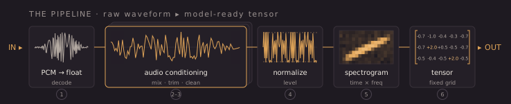
Raw audio is traced end to end, from an integer PCM buffer to the tensor the model sees. Each step does one thing, and every step between the endpoints is deterministic and shared.

Preprocessing pipeline: raw PCM decoded to float, a bundled audio-conditioning module covering mix, trim and clean, then normalization, a mel spectrogram, and a fixed numeric tensor. — The data's shape at each step: a raw waveform is conditioned in the audio domain, normalized, turned into a mel spectrogram, and resized to a fixed tensor. The audio-conditioning steps are bundled into one module. Illustrated on synthetic audio.

The Model

The classifier downstream of the pipeline is built on MobileNetV2, Google's lightweight convolutional vision network, adapted to audio through transfer learning in TensorFlow and Keras. The trick is treating sound as an image: the pipeline's mel spectrogram is stacked to three channels and resized to the fixed 224 × 224 tensor the network expects, so a model pretrained on ImageNet photographs can read time–frequency energy instead.

Starting from pretrained weights, the convolutional base carries over its general feature detectors and a new classification head is trained on the audio task. MobileNetV2's depthwise-separable convolutions and inverted residual blocks keep the network small and fast, which is what makes the single-command containerized inference service practical. The architecture stayed fixed across the ablation study below: with the model held constant, any change in behavior traces back to the preprocessing itself.

Experiments & Ablation

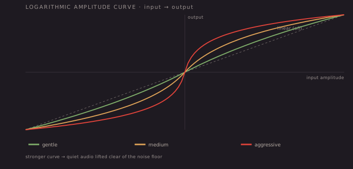
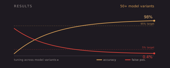
Beyond the pipeline itself, I ran a systematic study of how upstream audio preprocessing shapes model behavior. I trained 50+ model variants, each isolating a single preprocessing choice, to measure its effect on inference accuracy and false-positive rate, all applied on the waveform before the spectrogram was produced.

Logarithmic amplitude transfer curves at three aggression levels (gentle, medium, aggressive) against the linear reference; a stronger curve lifts quiet audio clear of the noise floor. — Amplitude-curve aggression, one of the swept dimensions. Left: logarithmic transfer curves from gentle to aggressive. Right: the effect on a signal, where a stronger curve isolates real audio from the noise floor before any spectrogram is computed. Illustrated on synthetic audio.

A tone burst before and after the amplitude curve: after the curve the noise floor is suppressed and the trace is cleaner and tighter. — Amplitude-curve aggression, one of the swept dimensions. Left: logarithmic transfer curves from gentle to aggressive. Right: the effect on a signal, where a stronger curve isolates real audio from the noise floor before any spectrogram is computed. Illustrated on synthetic audio.

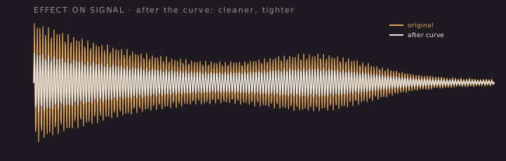
Every variant was run across three random seeds, so that any observed difference reflected the preprocessing change itself rather than the luck of a single initialization.

Impact

The result is a preprocessing path that is reproducible from a fresh clone and provably consistent between training and production. By making normalization stateless wherever possible and pinning the one stateful statistic to a single persisted contract, the pipeline eliminates an entire class of silent training/production mismatch bugs before they can reach the model.

Across the 50+ trained model variants, accuracy rises past the 95% target toward 98% while the false-positive rate falls below the 5% target toward 0.4%. — Tuning across 50+ model variants drove accuracy toward 98% and false positives toward 0.4%.

The work reflects how I approach ML engineering: treat the data path as a first-class system, make correctness structural rather than incidental, and document it so a team can build on it with confidence.

Adrianne with the engineering team in a conference room